Introduction
You’ve probably used prediction in everyday life without realizing it.
For example, imagine you’re browsing house prices –
1 BHK → ₹20 lakhs
2 BHK → ₹35 lakhs
3 BHK → ₹50 lakhs
Naturally, your brain starts estimating:
“What would a 4 BHK cost?”
You’re not guessing randomly — you’re identifying a pattern.
This is exactly what Linear Regression does.
what is Linear Regression?
At its core, Linear Regression is a supervised learning algorithm in machine learning used to predict a continuous value based on one or more inputs.
In simple terms:
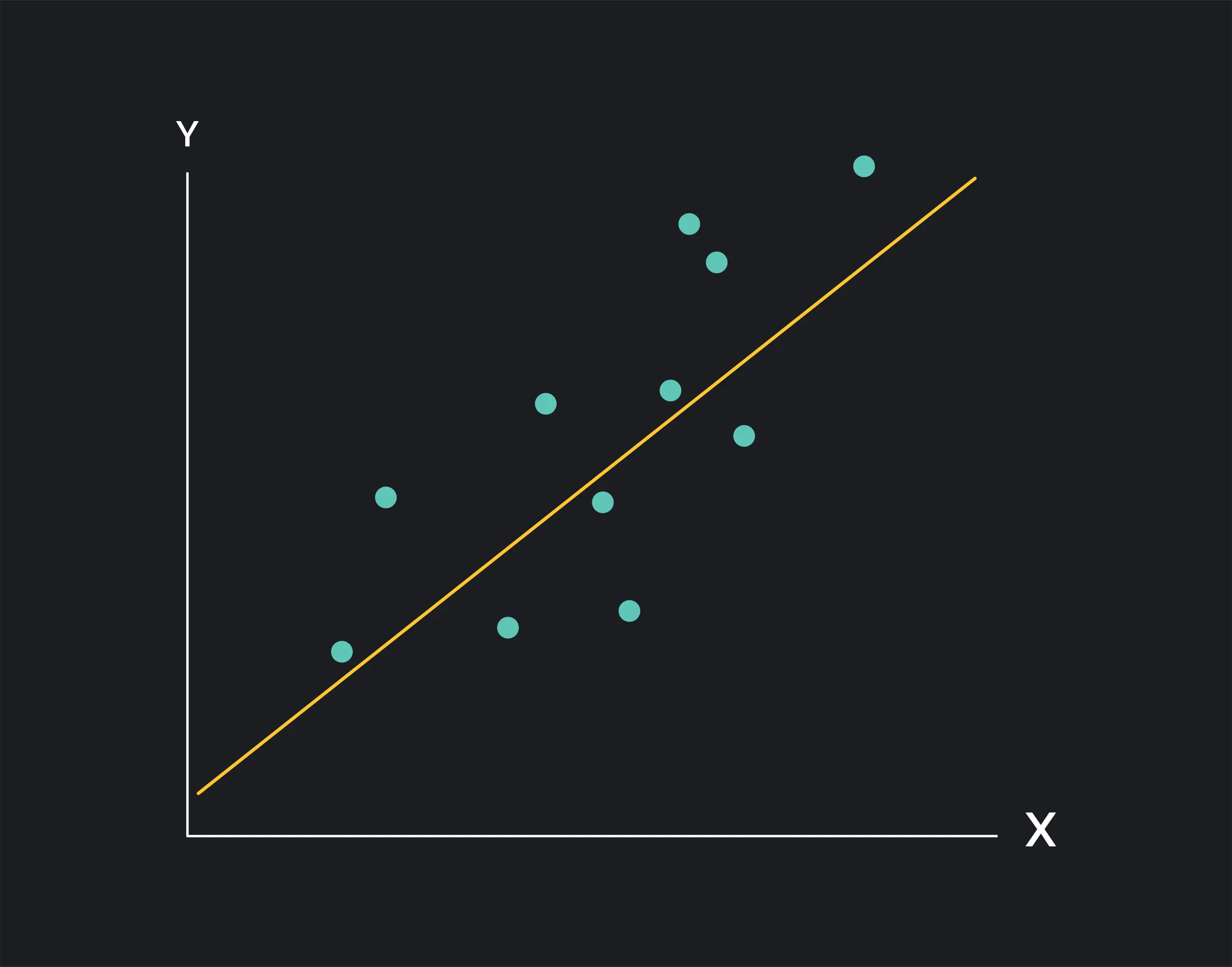
It draws a straight line through data that best represents the relationship between variables.
Instead of guessing prices manually, we can draw a straight line that best fits this data.
That line becomes our model.
Using it, we can predict:
“What will be the price of a 5 BHK?”
Understanding with an Example
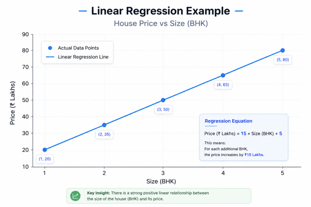
Consider the following data:
Size (BHK) Price ( lakhs)
1 20
2 35
3 50
4 65
If we plot these points, we notice an upward trend — as size increases, price increases.
The Equation Behind the Line
Linear Regression represents this relationship using a simple equation:
y = mx + b
where:
y is the predicted value (price)
x is the input (house size)
m is the slope
b is the intercept
with multiple variables(feature) the equation would look like this:
y = m1x1 + m2x2 + m3x3 + … + mnxn + b
What is the “Best Fit Line”?
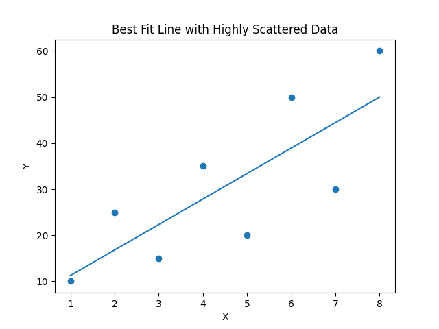
Not all data points lie perfectly on a straight line. So the model tries to find “Which line is closest to all the points?”
But here’s the important question:
How does it actually decide what “closest” means?
This is where model learning/training comes in.
Model Learning/training
To train the model, you feed the training set, both the Input features (X) — for example, house size (BHK) and the Output targets (Y) — for example, house price, to your learning algorithm.
The goal of the learning algorithm is to find a function that maps inputs to outputs. We represent this function as:
f w,b (x) = wx + b
(where w and b are called the parameters of the model that you can adjust during training, in order to improve the model)
This function takes a new input x and produces a predicted value, which we denote as:
y′
This y′ is the model’s estimate of the true value y.
Measuring Error
Once the model makes a prediction, we need to check how accurate it is.
For each data point, we calculate how far the prediction is from the actual value:
error = yactual – yprecticted
For example – house price prediction :
Size Actual Predicted
2 35 38
3 50 45
Now let’s calculate the error:
For 2 BHK:
35−38=−3
For 3 BHK:
50−45=+5
So the model isn’t perfect — and that’s expected. The goal now is to reduce these errors as much as possible.
“How do we measure the overall error across all data points?”
Looking at individual errors isn’t enough. We need a single number that tells us:
“How good or bad is our model overall?”
Cost Function
To measure total error across all data points. we square each error and then take the average.
This gives us the Mean Squared Error (MSE):
J(w,b) = 1/n ∑i=1n(yi−(wxi+b))2
yi → actual value
wxi+b → predicted value (y’)
n → number of data points
This function J(w,b) is called the cost function.
Goal of the model is to find the value of m and b such that the cost function is minimized.
Lower cost = better fit line
How Do We Minimize This?
We don’t try every possible line (that would be impossible). Instead, we use an optimization technique called Gradient Descent.
Gradient Descent : How the Model Learns
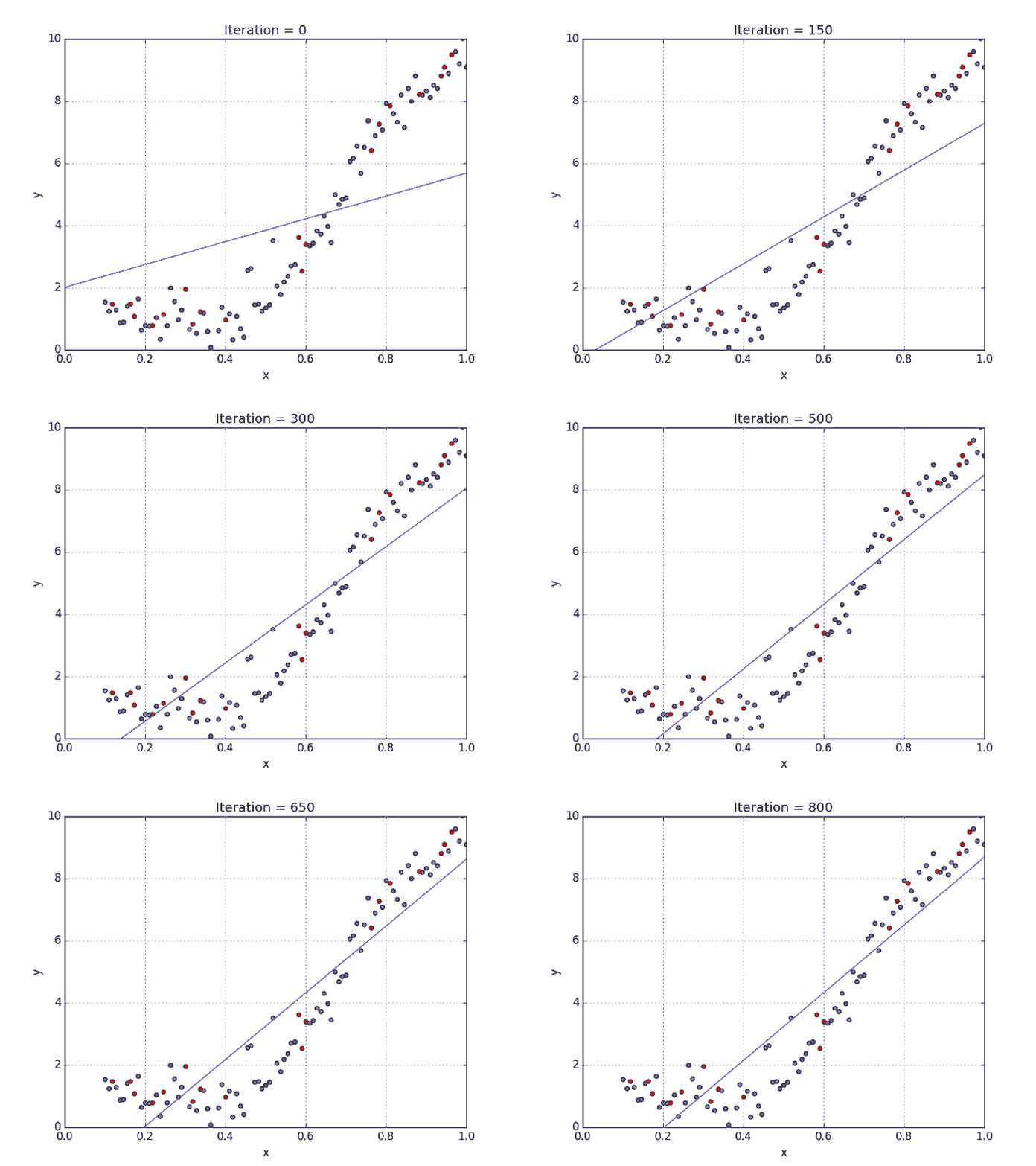
The idea is simple:
Start with a random line and keep adjusting it to reduce the cost J (w , b)
At each step:
- Compute the current cost.
- Check how changing and affects the cost
- Update them slightly in the direction that reduces the cost
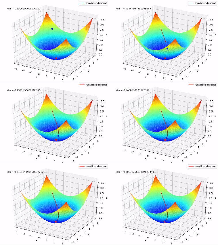
Intuition
Imagine you are standing on a hill in the dark.
Your goal is to reach the lowest point.
So you:
1. Take a small step downhill
2. Repeat
Eventually reach the point of minimum cost.
The Math Behind Gradient Descent
Recall our cost function:
J(w,b) = 1/n ∑i=1n(yi−(wxi+b))2
To reduce the cost, the model needs to know:
“Which direction should I move to decrease the error?”
This is done using derivatives.
A derivative tells us:
If a value changes slightly, how much does the output change?
So:
∂w/∂J -> tells us how changing affects the cost
∂b/∂J -> tells us how changing affects the cost
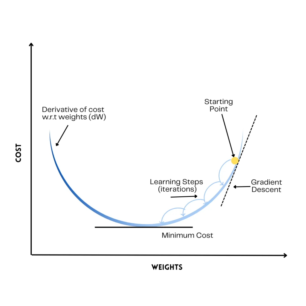
If , increasing increases the cost, so we move in the opposite direction.
If , increasing decreases the cost, so we continue moving in that direction.
The parameters are updated on each iteration using:
w = w − ∂w/∂J
b = b − ∂b/∂J
Here, is the learning rate, which controls the step size during learning.
Large → takes very big steps and may miss the minimum point
|Small → takes tiny steps, so learning becomes slow
The algorithm iteratively makes predictions using the current line, measures the error, computes the derivatives, adjusts w and b, reduces the cost, and eventually converges to the best fit line.
That’s it for this one. Hope this made Linear Regression a little less intimidating 🙂
see you in the next blog

Leave a Reply